해당 강의는 나머지 뒤의 수업에서 전반적으로 다루어질 특정한 몇 개 분포에 대하여 빠르게 리마인드하고 moment - generating function, law of large numbers, central limith theorem들을 컨셉과 증명을 이해하는 것을 목표한다.
Lecture 3. Probability
Random Variable
Discrete X, continuous Y
Prob mass function f_x, prob density function f_y
f_x: sample space -> R > =0
sum of f_x(x) = 1, (x in sample space)
Prob of event
- P(A) = sum of f_x(x), x in A
- Expectation E[x] = sum of x * f_x(x)
Independence
mutually indep - consider in this lecture
- whatever we collect are independent
pair wise independent
Log - Normal Distribution
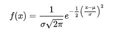
Continuous random variable has
normal distributionif its probability density function is![]()
주식 가격을 모델링할 때, 시간에 따른 가격의 편차를 Normal로 가정하여 모델링을 수행하는 것은 옳지 않을 때가 많다. 일반적으로 추세가 존재하여 평균이 시간의 흐름에 따라 일정하다는 가정이 어긋나기 때문이다. Instead we want the “relative difference” to be normally distribution
- (P_n - P_n-1) / P_n ~ N(0,1) – Percentage Statistic
- 그럼 가격 변동 비율이 위의 분포를 따를 때, 가격 P의 분포는 어떻게 될까?
(Thm) Change of variable
Suppose X,Y are random variables such that P(X<= x) = P(Y <= h(x)) for all x
Then f_x(x) = f_y(h(x))* h’(x)
X: log-normal distribution, Y: normal distribution일 때 위의 정리를 통해 x의 pmf 를 구할 수 있다.
해당 pmf 역시 기존 Y의 mean μ, std σ를 parameter로 갖지만 더 이상 평균과 분산을 의미하지는 않는다.
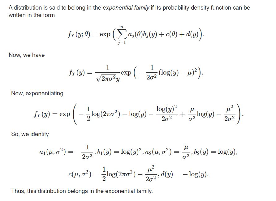
Exponential family of distribution
A distribution belongs to exponential family if some vector θ that parametrized distribution such that
f_θ(x) = h(x) * c(θ) * exp(∑ w(θ) * t(x) ) == 확률 함수가 (x,θ,exp(x,θ))로 구성된다.
log - normal distribution 역시 exponential family 중 하나이다.
![]()
수업 청강하던 다른 교수님 코멘트
The notion of independent random variables, you went over how the probability denstiy functions of collections of random variables if they’re mutually independent the product of the probability densities of the individual variables. And so with this exponential family, if you have random variables from the same exponential family, products of this density function factor out into a very simple form. It doesn’t get more complicated as you look at the joint density of many variables, and in fact simplifies to the same exponential family. So that’s where that become very useful.
Exponential family가 가지고 있는 강점은 여러 분포의 확률 함수를 일정한 폼을 가지고 있는 factor들로 분리 할 수 있다는데 있다. 여러 분포의 결합 확률 분포가 다루기 좋은 exponential family의 factor 형태로 얻어지기 때문에 활용이 용이하다.
Moment Generating Function
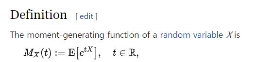
- mgf를 t에 대하여 k번 미분하고 t에 0을 넣으면 random variable의 k 번째 moment를 얻을 수 있다.
- Random Variable의 k번째 moment가 의미하는 것은 r.v에 power k한 것의 기대값이다.
모든 r.v가 mgf를 갖지는 않는다. (ex) log-normal distribution
(Thm 1) If X,Y have the same mfg the X and Y have the same distribution
위 정리가 X,Y가 모든 k에 대하여 X^k == Y^k를 갖는다고 하여
두 r.v가 같은 분포를 갖음을 보장하지는 않는데
두 r.v의 mgf가 존재하지 않는 경우도 존재하기 때문이다.
(Thm 2) X1,X2, … Xn is a sequence of r.v such that Mx_i(t) converge to Mx(t)
for some r.v X for all t, Then for all x P(X_i <= x) converge to P(X <=x)
- mgf가 converge하면 분포도 converge 한다.
Large Scale Behavior
해당 수업의 관점에서는 Large Scale Behavior란 Long Term Behavior라는 것과 같은 것으로 볼 수 있다. 하나 하나의 random variable에 대해서는 어떤 값이 얻어질 지 예측할 수 없다. 그러나 분포가 같은 여러 independent random variable을 함께 묶어 모델링을 수행하면 특정한 분포를 보일 것이라 추정할 수 있기 때문이다.
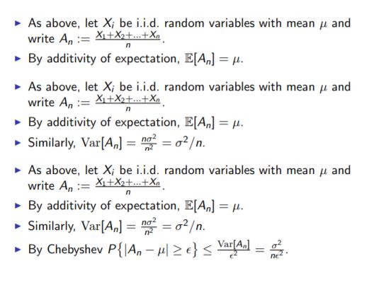
Law of Large Numbers
(Thm) Week Law of large numbers
Let X1,X2, … Xn be variables with i.i.d ~ (μ,σ)
Let X = (X1 + X2 + … Xn)/n, then for all ε>0, P(abs(x-μ) >= ε) converge to 0 as n becomes infinity
그런데 위의 정리의 증명을 볼 때, ε를 0.01로만 놓아도 조건을 만족하기 위해 n이 아주 커져야 하는 것을 알 수 있다. 따라서 위의 정리에는 week law라는 이름이 붙은 것이고 수업에서는 언급되지 않았지만 strong law of large numbers도 물론 존재한다. 궁금하다면 여기에서 자세한 설명과 증명을 볼 수 있는데, 필요한 조건이나 증명의 복잡성은 물론 week law보다 더 필요하다.
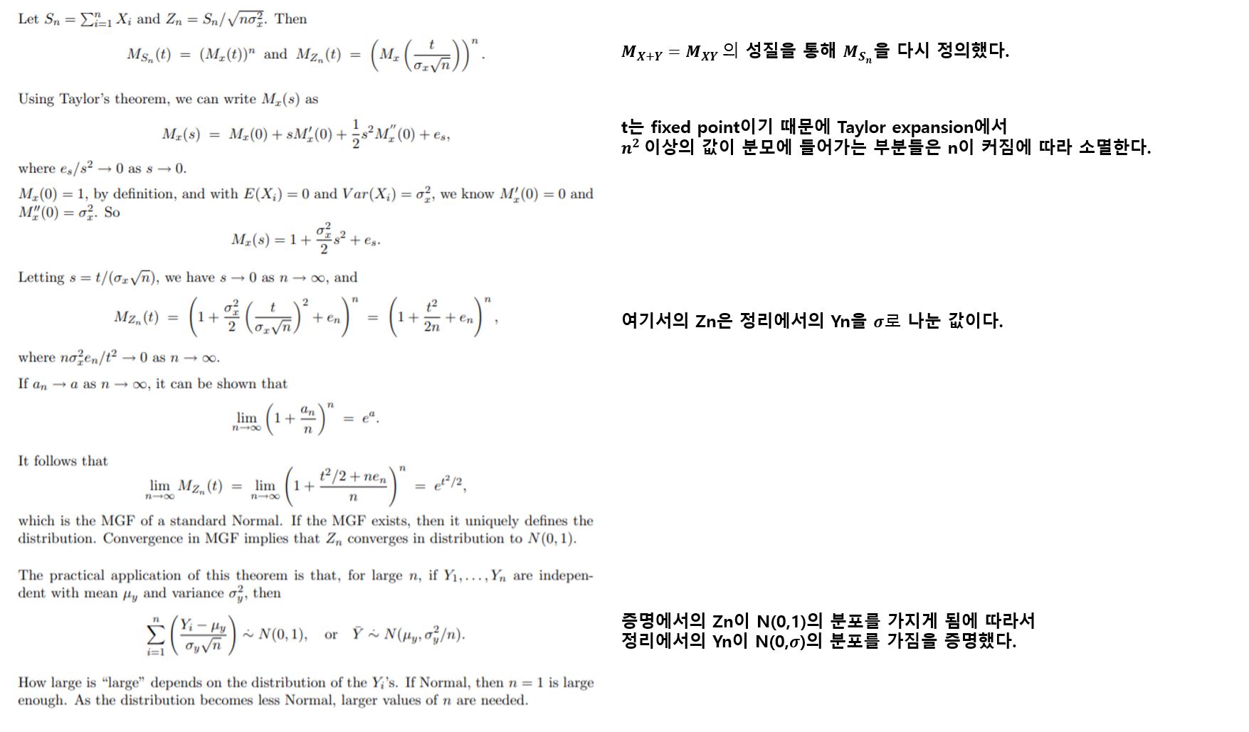
Central Limit Theorem
(Thm) Central Limit Theorem
Let X1,X2, … Xn be variables with i.i.d ~ (μ,σ)
Let Yn = ∑(x_i - μ)/sqrt(n) then the distribution of Yn converges to that of N(0,σ^2)
For all x, P(Yn <= x) converges to P(N(0,σ^2) <= x)
CLT는 random variable의 mgf가 존재한다는 가정에서만 증명 가능하다.
CLT에 대한 증명에 앞서 N(0,1)의 mgf를 구하는 과정을 먼저 본다.
![]()
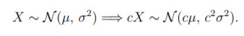
또한 평균이 0일 때, N(0,σ^2) == σN(0,1)라는 것도 알고 있자.
![]()
![]()

선형대수와 수리 통계의 내용 중 뒤의 강의를 이해하기 위한 핵심적인 수학 이론들에 대해서 리마인드하였다. 수업 사이 사이에 매트릭스나 분포 formula를 어떻게 주식 모델링에 적용할 수 있는지 간단하게 설명해주는 것이 재밌었다.